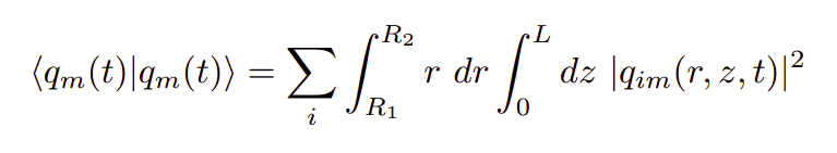
The basic work has been completed and the results are now available. As discussed earlier after applying the Fast Fourier Transform along the azimuthal direction, we calculated the covariance matrix of the velocity fields together.
The motion is described by the very famous Navier-Stokes equation. This is a nonlinear partial differential equation which makes them interesting and challenging at the same time.
We have generated data from the quasilinear simulations of the equation through pseudo-spectral methods. The data collected is for every point in space and time, and is a 4-Dimensional, which includes three scalars representing the velocities along the axis, along the radial and tangential directions along with the scalar pressure component.
We construct the covariance matrix and analyse the eigenvalues at each wavenumber, since we apply a fourier transform over the azimuthal dimension. Before plotting we clip the values in a appropriate range as maintaining values beyond 15 orders of magnitude is not useful. Various colormaps and scales are used for plotting, we use a logarithmic scale, and also look at the values ignoring the first value which is quite high in value. The energy is concentrated in the first mode which is as per our expectation.

The data I have been working so far was the one obtained from the quasi-linear simulations of the Navier-Stokes Equation. The transitional state of flow was considered so far. This is where we would be able to see some pattern of the energy distribution in the modes. We are yet to have the same plots for the fully turbulent state which would be the most exciting ones.
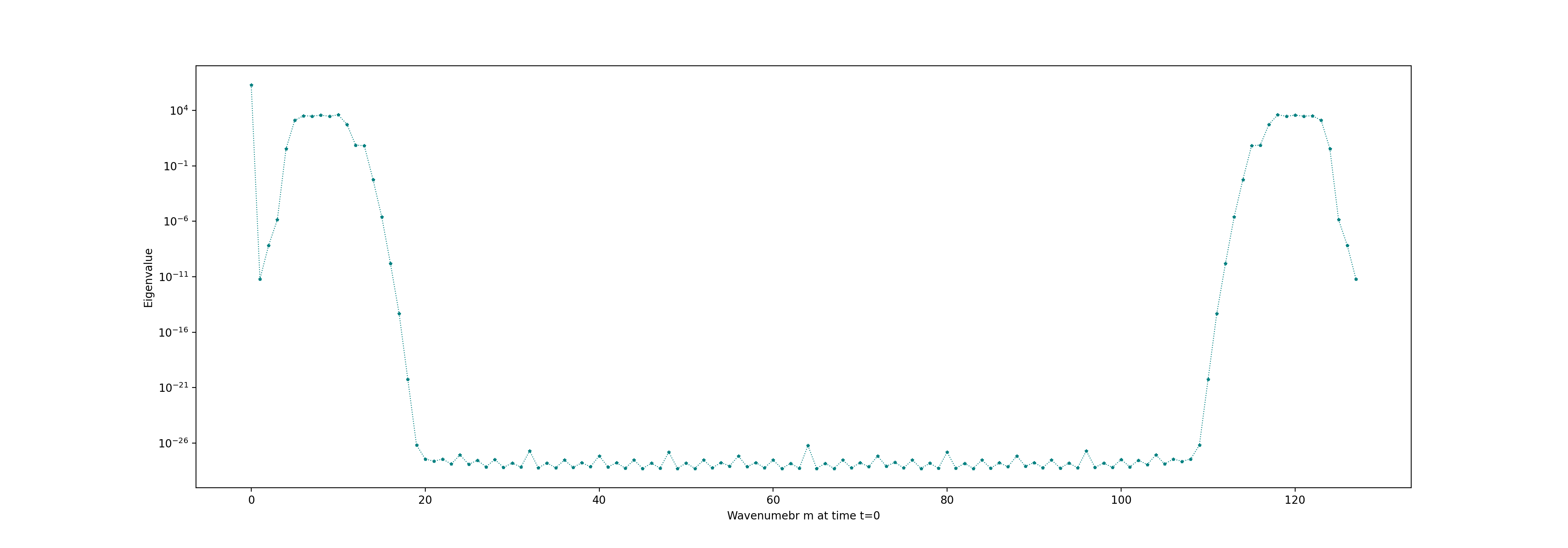
The values here are plotted on a logarithmic scale and we can notice aliasing as the plots are symmetric about the mid input