Now that we have the results for the azimuthal direction averaged covariance, we consider going one step further by applying Fourier transform (FFT) along both the azimuthal and the axial directions. Now we would have one eigenvalue for each mode k_z and m, which means we would have to employ different strategies to plot the eigenvalues.

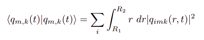
Here as we have a fourier transform over the axial direction, the outer integral vanishes as compared to what we had previously
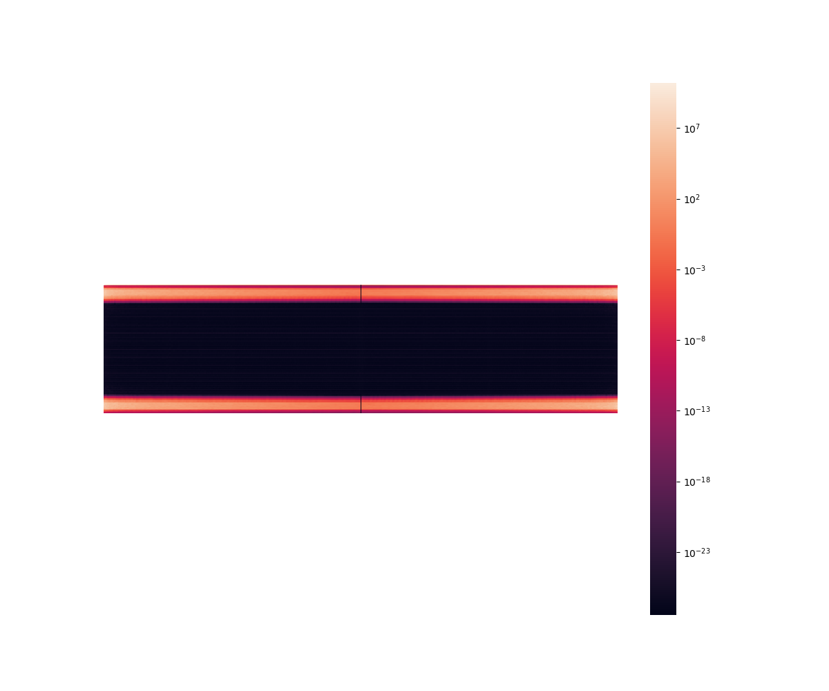
Since the input space is now 2-dimensional, it is natural to have heatmaps as below. But we don’t get much information through them.
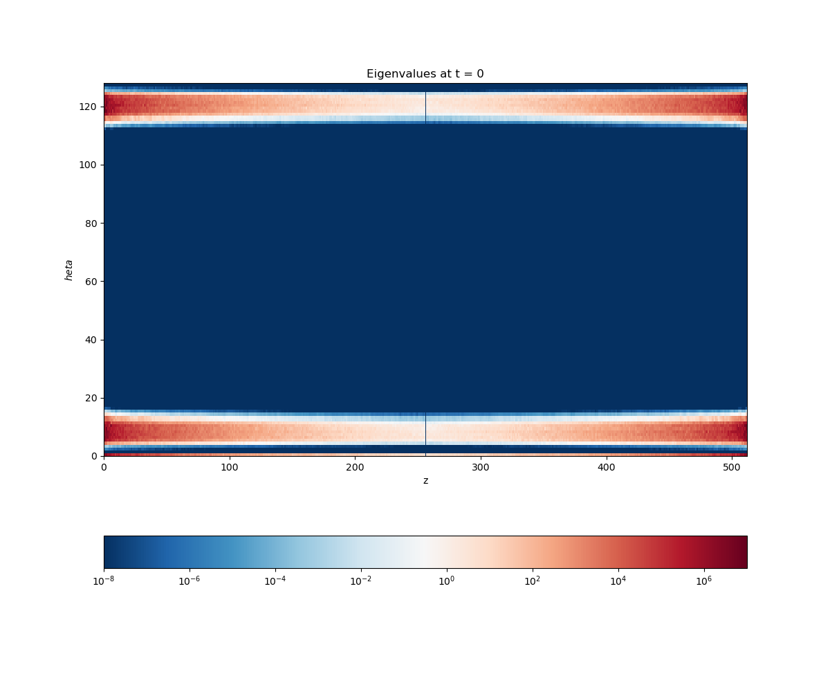
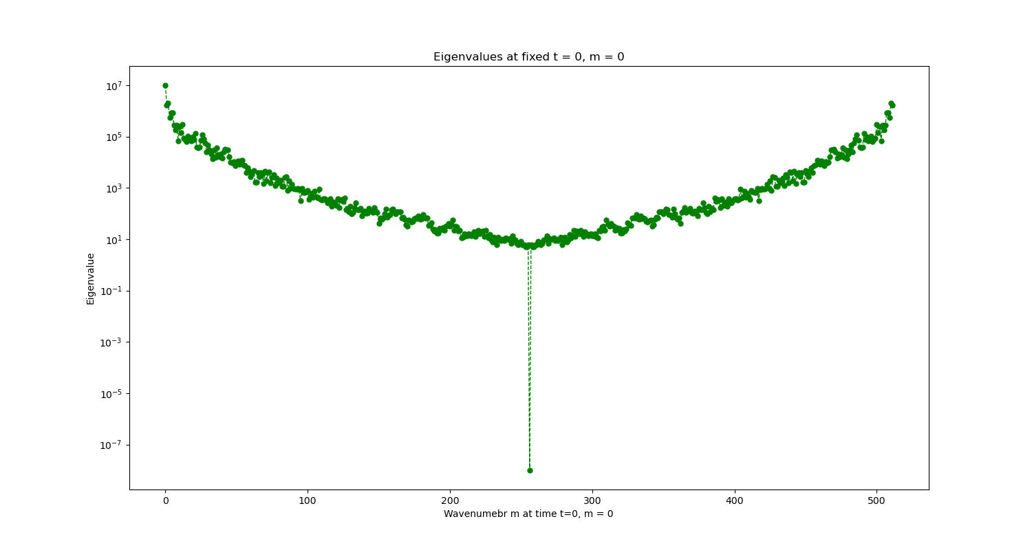
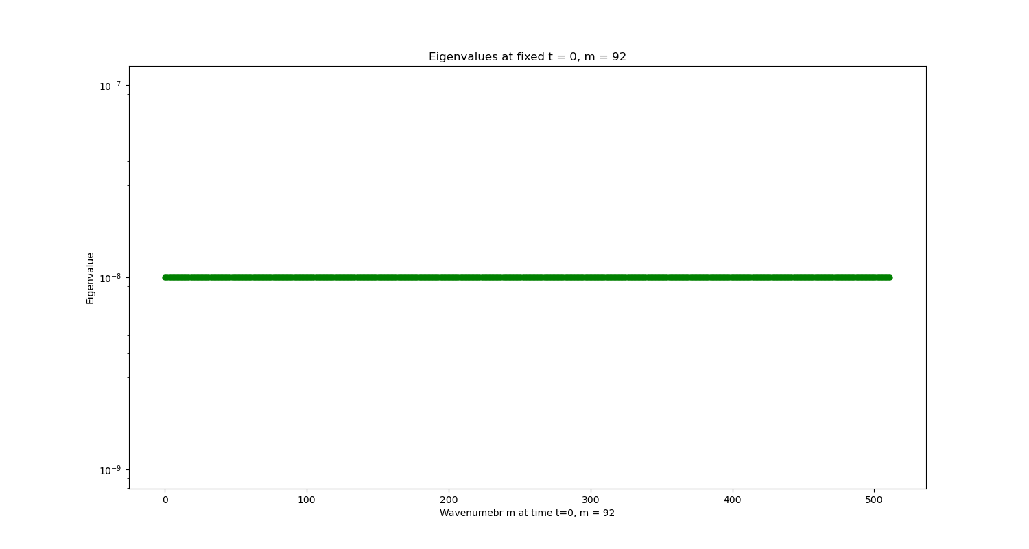
We plot each ‘vertical slice’ and ‘horizontal slice’ of the heatmap, which implies we fix one of the wavenumbers, either k_z or m and plot the variation of the eigenvalue against the other varying wavenumber
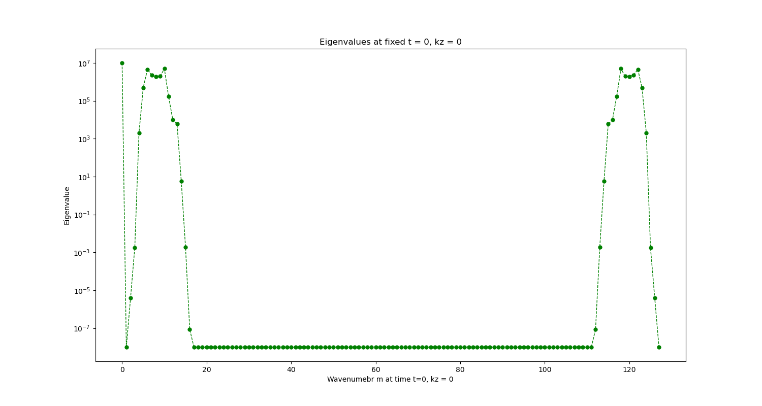
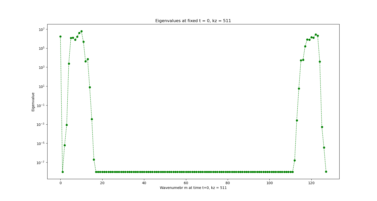
Here we keep the azimuthal wavenumber constant and vary the axial wavenumber. We notice certain flat lines in the graph, they correspond to the values which got clipped off as they were too low and are not worth considering for any practical purpose
The final clean plots for the completely turbulent and fully laminar flows are yet to be finalized and I would be getting through them soon. Now what remains is looking at the plots carefully, analysing some particular modes and reconstructing the data through some select modes Another technique we would like to explore is Deep Learning for Unsupervised Learning. Naturally, autoencoders offer an efficient solution to the problem of transforming the input feature space.
>